Dexter Industries IMU, part II

Last time I reviewed the gyro of Dexter Industries IMU sensor. This time I’ll take a look at the accelerometer of the IMU. I’ll compare this one to the MindSensors accelerometer and to the one on my custom IMU.

The three accelerometers in the test all all 3-axis digital sensors that support hi-speed I2C. They all allow you to set dynamic range, the MindSensors sensor supports 1.5, 2, 4 and 6G. The dIMU supports 2, 4 and 8G and my cIMU supports 2,4,8 and 16G. On the NXT you would normally use 2 or 4G dynamic range.

I tested the sensors at 6 and 8G. The resolution (the minimum difference between to samples) of the Mindsensors accelerometer is 1 milli-G for all ynamic ranges, the dIMU and the cIMU both have 16 milli-G at 8G. The MindSensors sensor has the best resolution. Later, I’ll explain why.

The test protocol is very simple. The sensors are tested at the same time. First they are horizontal, then they are tilted manually to an angle of 90 degrees and then they are turned back. The test tells something about the accuracy and noise levels of the sensors.

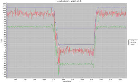
The first graph shows the unprocessed output of the Z-axis of each of the sensors. You would expect a value of 1000 milli-G when the sensor is horizontal and 0 milli-G when tilted. As you can see in the graph the three lines are quite different. The MindSensor gives smooth output with little noise. My sensor is very noisy, the line goes up and down. And the dIMU has some noise. What is more, the three lines are on different heights and none is on the expected level. Apparantly the sensors need calibration, to get the lines on the expected level, and the two IMU’s need some smoothing as well. My IMU allows to set the internal sample rate, lowering this to 100 Hz removed some of the noise. In later tests I used the lower sample rate.

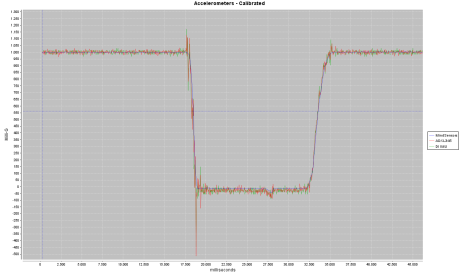
Calibration of accelerometers is quite easy. The MindSensors sensor has an on board calibration routine but I advise you not to use it and to write your own instead (or use the program that MindSensors provide on their website). Calibration consists of determining an offset and a scale factor. The offset is a value that you substract from the raw value. It is equal to the value the sensor returns when it experiences zero G. For the MindSensors sensor used in the test this is about 125 milli-G. For the other two sensors it is a lot harder to find the offset value as the returned values are not stable at all. One has to take the average of multiple measurements to find the offset. Offset values of accelerometers are quite stable, once you found it you can keep using it. But keep in mind that each of the axes has its unique offset value.Then there is scale. After an offset correction has been applied to the signal one gets a zero at zero gravity conditions. This does not mean that one gets 1000 Milli-G under earth’s gravity. Normally this is a few percent off. A scale factor can correct for this. The scale factor equals 1000 divided by the offset-corrected-value the sensor returns under earth’s gravity. The formula to get a calibrated acceleration signal is:
value=(raw_value-offset) * scale
That’s all there is to it. Scale too is quite stable. You can hard code it in your programs once you calculated it. You’ll have to calculate it for each of the axes though. The next graph shows calibrated output of the three sensors.
Apart from the noise levels, all sensors perform very well after calibration.

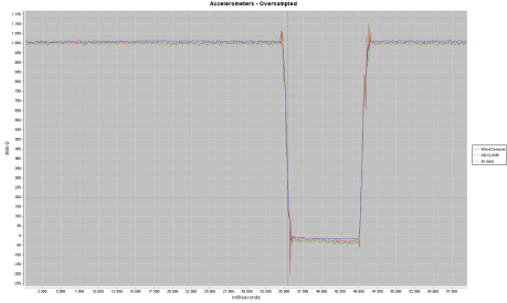
The MindSensors sensor has a lower noise level and a better resolution than the other two sensors. This clearly is a big advantage of this sensor. But how come this sensor is so good? I suspect it is not the sensor itself but some on board filter that stabilizes the signal. Therefore I decided to write a filter for the other two sensors as well. At first I tried a low pass filter as this is very easy to program and uses little memory, but this filter added a delay in the response, so I abandoned this idea. Then I tried a technique called over-sampling. Basically this means that one tries to get measurements as often as the sensor allows and then calculate a moving average from it. This did the trick, the noise levels of both IMU sensors dropped dramatically and the resolution rose. Both IMU still are more noisy that the MindSensors accelerometer, the difference however is acceptable.

Of course a filter like this does come with some extra costs. One has to program it, It will have to run in a separate task, so that your program can still do the other useful things it is meant to do. And the filter consumes processor time.

The test I perormed was limited and not scientifically sound. However I conclude that all sensors perform well under test conditions. The MindSensors accelerometer is the best accelerometer for most of us as its signals are most easy to use. It does not have a gyro sensor on board as IMU sensors do. So if you also want a 3-axis gyro then you should consider an IMU sensor. The price dIMU is just 15$ more than the MindSensors accelerometer. This could be a good reason to go for the IMU straight away.

The IMU sensor filter, part III

In a previous post I showed how the Filter for the IMU sensor combines both gyro and accelerometer data to get drift-free low noise information about the robots orientation in space. The filter performs a second function, it translates sensor output to a world frame of reference. In this post I’ll explain what I mean by that and how the filters works in this respect.

Body frame of reference versus the world frame of reference

Suppose you are standing upright facing north when somebody next to you asks you to turn right for 180 degrees. After you turned so you’ll be facing south. Clear enough. Now suppose you are lying on the ground face down and head pointing south. If you are asked again to turn right for 180 degrees by the same person you will have to consider two options regarding the meaning of the word right. The first option is that right should be in reference to your body. If you turn like this you’ll end up face up while still pointing north. The second option is to treat right in reference to the person that asked the question. If you turn like that you’ll end up still facing down but with the head pointing south.

The same goes with robots and the sensors they carry. Your robot might have a gyro that indicates that the robot turns clockwise, but if the robot is upside down you’ll see itt turning counter clockwise. This is because the robot and the gyro attached to it have a different reference than you have.
To distinguish between the two references we call the first one the body frame of reference and the second the world frame of reference. The world frame of reference is supposed to be inert, a global frame where everything can relate to. Words like up, down, north and south are related to the world frame of reference. The body frame of reference belongs to the robot and the sensors. When the robot moves its body frame of reference moves along with it. Robot commands like drive forward are always in respect to the body frame of reference. Likewise, data from the sensors are also expressed in the body frame of reference.
In robotics, you’ll frequently have to translate information from one frame of reference into the other. For example, when you calculate the position of the robot (world frame of reference) from data from the tachometer (body frame of reference). The process to translate information from one frame to another is called transformation.

Transformations

A transformation requires the use of trigonometry. Suppose again that you want to calculate the position of the robot (world frame of reference) from data from the tachometer (body frame of reference). Let us assume that the tachometers indicate the the robot has travelled straight forward for 30 cm. In terms of body frame it is said that it moved over the x-axis with 30 cm and over the y-axis with 0 cm. Suppose the robot was facing east when it travelled and you have called the east to west axis the y-axis as is customary. It is clear then that in the world frame of reference the position of the robot increases by 30 cm along the y-axis and maintained its position along the x-axis. In mathematical terms the transformation from body frame to world frame is:

Xw = Xb * cos(a) - Yb * sin(a)
Yw = Xb * sin(a) + Yb * cos(a)

Where the parameter a stands for the angle between the robot (or better the body frame of reference) and the world. In the above example a=90, making cos(a)=0 and sin(a)=1. as a result the x and y values are swapped in the transformation.
Transforming sensor output to world frame of reference is the second function of the IMU filter. However, It does so in a 3D space and not in a 2D space as the example.

The preferred way to model a transformation mathematically is by using matrices and vectors.

This is the preferred way as it offers a convenient and short way to describe both the transformation and sensor output. Without going in too much detail, the transformation is stored in a transformation matrix of 3 by 3 elements. The sensor output is stored in a vector of 3 elements. To transform a vector from body frame of reference to world frame of reference one has to execute a matrix multiplication on the body vector using the transformation matrix. In mathematical terms:

Vw = Vb X T

Where T stands for transformation matrix. To go from world to body the formula is:

Vb = Vw X  Tinv

Where Tinv represents the inverse matrix of T.

Internally the filter maintains a transformation matrix. The robots current attitude can be calculated from the transformation matrix.

The IMU sensor filter, part II

Here a quick post of some graphs that show the effect of the filter I use for my IMU.

You might have seen a previous posts where I show you that my sensor is capable of detecting a grain of sugar under the NXT. If you haven’t seen it, check the post and video here. Few months ago I changed from robotC to Lejos. And now I have rewritten the sensor drivers and the filter in Java.

The Lejos developers are currently working on a very nice logging feature that allows users to display data from the NXT real time on the pc. I got hold of the beta code and tested it without any problems. I used the NXTDataLogger (this is the name of the Java class) to made the intrinsics of the IMU filter visible.

The IMU sensor combines a 3-axis gyroscope and a 3-axis accelerometer. The filter reads the output from both sensors, combines there signals in a smart way and provides stable information about the orientation (yaw, pitch and roll) of the robot.

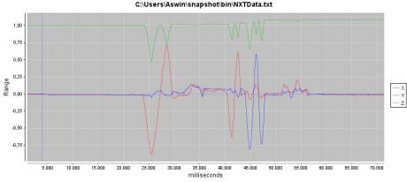
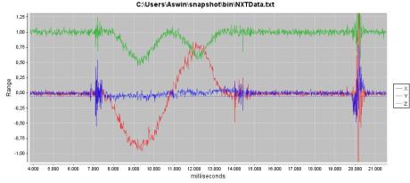
An accelerometer can provide tilt data (pitch and roll) as can be seen in the first graph. This sensor however has two serious drawbacks. First it is quite noisy, that’s why the graph lines seems so hairy. Second, it does not distinguish tilt from acceleration. So, the output from this sensor can have different causes. This is why you cannot make a balancing robot with just an accelerometer.

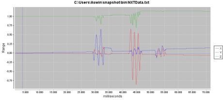
A gyroscope is far less noisy, that is why the second graph shows smooth lines. It is also not affected by acceleration. However also this sensor has its particularities. First, it doesn’t measure tilt, but it measures rate of turn. This can only be translated into tilt if the starting condition is known. To get the tilt at any time you have to integrate all the readings and the starting condition. In the process small errors are introduced, in the long run they add up to la large error. The green line in the graph shows this effect. At about 42 seconds the sensor rotates faster than its maximum range (>2000 degrees/second), it then gives faulty readings, these are integrated in the calculated tilt. As a result the line ends higher than it started, even though the sensor was turned back to its original position. The second effect that makes a gyro hard to use in long runs is called drift. Due to temperature changes or voltage drops the base level of a gyroscope changes. This means that after some time the gyro seems to be turning slowly when it is still being stationary. This effect is well visible in the blue line. This goes up slowly. This effect can not be eliminated by calibration, unless you are able to calibrate the sensor along the run.

The filter is like a PI-controller. It uses the data from the gyroscope as the basis of it’s output. The lines in the third graph, that shows the output of the filter, are smooth because of this. It uses the data from the accelerometer to correct the output from any errors that have been build up. But it does so slowly in order to keep the noise out of the output signal. The P-value of the PI controller corrects for errors in the gyro signal. It also makes the filter usefull when starting conditions are unknown. The filter also sums past errors to get an I-value, this value is used to correct for drift in the gyro data. The result is a graph with smooth drift-free lines.

Two final notes. First, the green line (the yaw-line) is not drift-free. This is because an accelerometer cannot provide information of orientation in the XY-plane. You need a compass sensor to provide this information. Second, the range is expressed in cosine of the angle, so 1 corresponds to zero degrees, 0 corresponds to 90 degrees.

Calibration of the accelerometer

An accelerometer can be a very useful sensor for your robot. It measures acceleration or changes in motion. Most available sensors do this for 3 axis. Acceleration can be used to calculate tilt, movements, changes in speed and changes in position.

An accelerometer measures earth gravity too, a motionless sensor still reports an acceleration on the Z-axis of 1G (=9.81 m/sec^2). Thanks to earth’s gravity a motionless accelerometer can be used to calculate the tilt angle of the sensor. The acceleration (in G) that an accelerometer measures on each axis equals the cosine of the angle that the axis makes. This angle is in respect to a vector that is pointing straight down. When the accelerometer is accelerating, for example because your robot is going from stand-still to a motion, you can no longer calculate tilt angles reliably. But once the robot is in a constant motion you can. Some accelerometers, like the mindsensors accelerometer, can report tilt angles directly. But I think it is best to calculate it yourself from the acceleration as this is often more precise.

From the acceleration you can calculate speed, and from speed you can calculate position. Well, to be precise you can only do that if you know initial speed and position. As we normally do not build air-to-air missiles, we can assume the initial speed of our robots is zero. That is also what we assume for initial location.
A simple way to calculate the speed from the acceleration is to take the last known speed and add the acceleration (in m/sec^2) times number of second (since the last known speed was calculated). This process is called integration. It assumes that no big changes in acceleration have occurred between the two measurements. The less time that there is between two measurements the more likely this is to be true. Therefore it is often a good thing to have your sample rate as high as possible. To calculate position you have to integrate speed. Thus location = last location + speed * seconds since last time. This is called a second order integration because speed itself is the result of an integration.

During integration small errors in measured acceleration build up quickly. Suppose your sensor reports an acceleration of 1 milli-G where as in reality this is zero. After just one minute this small error results in a calculated speed of 59 cm/sec^2 or 2 km/hour. In a second order integration errors build up even faster. An error of one milli-G is much smaller than the error of the accelerometers we use. It is even smaller than the resolution of the sensors we use. Resolution normally is around 3 milli-G. This makes it impossible to get a reliable speed or position from just the accelerometer. But still acceleration can be of use for this in combination with other sensors like a GPS or wheel tacho’s. It can replace a GPS for a short time when there is no GPS signal. Or it can help to detect wheel slippage and correct for this.

If you want the best possible information from your sensor you need , as always, to deal with three aspects. Calibration, sensor mounting and sensor noise.

Calibrating an accelerometer minimizes the internal error of the sensor. There are, at least, three kinds of internal errors in accelerometers. Offset, scale and linearity.
Offset error means that your sensor reports too high, or low, consistently. This can be dealt with easily. The sensor value you get from a motionless sensor equals the offset error. On the Z-axis you’ll have to correct for gravity though.
Scale error means that the sensor reports a value that is a certain percentage of the actual acceleration, even when the offset is right. The scale error can be easily calculated as well thanks to gravity. It takes two measurements to calculate the scale, one while pointing the sensor straight down and one while pointing straight up. You know that the difference between to the should be 2 times G.
Linearity error means that the sensor is not consistent over its range. Or put it differently, the scale error differs with different magnitudes of acceleration. linearity errors are hard to overcome. Luckily the dynamic range of NXT robots is really small, you can therefore can ignore linearity errors.

Sensor mounting is the aspect you’ll have to deal with when you want good sensory input. A misaligned sensor will report faulty values. Suppose your sensor points down with 45 degrees your sensor will report an acceleration of 0.7 G when there is none (excepts earths gravity). If your robot is only free to move upright on a flat surface you can prevent these errors with careful construction. So in most cases this aspect can be ignored in software. If however your robot has freedom of tilt you must deal with this in the software. But this is not considered an error and won’t be discussed in this post.
Moving robots vibrate. These vibrations are also measured by the sensor and make the signal more noisy and harder to interpret. It is a good idea to mount your sensor somewhere were the vibrations are the least powerful. Do not mount it to high or on one side of the robot. As a rule of thumb, the best place is on the center of gravity or straight below it.

The third aspect is sensor noise. I do not mean noise due to vibrations as discussed above but the noise that is in the electronics itself. Don’t we all get tired with sensor noise? Accelerometers are particularly noisy. I won’t bother you with statistics and noise measurements this time. Take a look at the output of your sensor to get an idea. You’ll see values that are more then 5% of the expected value quite frequently. You’ll have to take noise into account when calibrating your sensor. Do not rely on a single measurement but take the average of multiple (400) measurements to eliminate noise during calibration. Most sensors have some internal ways to minimize noise. Most often this is done by a low pass filter, sometimes you can even tune this filter. You can always make your own low pass filter to get the noise levels even further down. But remember, a low pass filter makes your sensory output less responsive, it takes some time for real changes to be visible in there full extend.

 

The Mindsensors accelerometer is the most common accelerometer for the NXT. It has I2C commands to calibrate the sensor, Mindsensors also provides a program to calibrate it. The commands are quite cumbersome to implement. The program is easy to use, but you need to have the standard firmware to run it. You can also write your own calibration routine, this is not as hard as it may seem. There is one disadvantage though, the calibration settings are not stored in the sensor and need to be included in your programs. If you want to write your own calibration program, here is how.

1. Make a function that returns the uncalibrated (raw) values.
2. position the sensor in such a way that the axis to calibrate is pointing straight down. It doesn’t have to be spot on, a few degrees of do not matter very much.
3. take the average of a number of raw sensor values and store/remember this as the minimum value.
4. position the sensor straight up.
5. take the average of a number of raw sensor values and store this as the maximum value.
6. take the average of the minimum and maximum values. This is the sensor offset, it is used later to calculate calibrated values.
7. take the difference between the minimum and maximum values. This range represents 2 G’s.
8. divide the range by 2000. The result is the scale factor you need to get calibrated readings in milli-G.
9. repeat this process for each of the axes.

Knowing both the offset and the scale factor you can now calculate a calibrated value from a raw value. Take the raw value, subtract the offset from it and multiply by the scale factor.  The result is a calibrated value in milli-G. Just to make sure you understand, all three axes have their own offset and the scale factor.

Offset and scale do not change over time , so once you get these values you can hard code them in your programs. There is no need to calculate these values every time you run your program.

From robotC to Java

It has been sometime since you saw a post from me. The main reason is that I am really busy with work. The second reason is that I decided to use the LEJOS environment for my current project. I did not have any experience with LEJOS and Java, so I had to dive deep into the matter.

LEJOS allows you to program in the Java language on the NXT. It has some advantages over robotC that I have been using the last two years. I won’t list all the differences between the two languages. For me the higher I2C speed and object orientation were important factors.

Java proved to have a steep learning curve. It took me some time to get the first results. The main reason for this was not the language itself but the IDE. I am using Netbeans to write my programs. Netbeans uses ANT to compile the programs. ANT uses the classes provided with LEJOS. All these components have to work together. And when they don’t it is hard to find out why for a newbe like me. At one point I experienced lots of red lines in my program, indicating errors, but still the program compiled just fine. It turned out that ANT did know where to find the LEJOS classes but Netbeans didn’t.

Slowly I’m getting to grips with Java and the environment. As a first project I decided to write an improved interface to the Mindsensors accelerometer as the existing  interface does not allow to set the sensitivity of the sensor or to calibrate it. I also want my sensors to return SI values, I rather have m/s^2 than milli-g for acceleration, I rather have radians than a number between -127 and 128 for tilt. The interface is no jet finished but I do not feel lost anymore when writing a new method to the interface.

After I finish this little side-project I will rewrite the interface to my IMU and the component filter. Only then I can really tell whether my switch to LEJOS has payed of.

A grain of sugar

I totally forgot to post the video I made of the IMU sensor.

This clips shows how accurate the IMU sensor can be. This IMU sensor combines a 3 axis gyro and a 3 axis accelerometer. The signals from both sensors are combined using a nonlinear complementary filter to get an output signal that has low noise and is drift free. (Well actually it is only drift free over 2 axis. It still drifts over the Z-axis.) This home made sensor will show a blue light when it is horizontal using a 0.5 degrees margin. Otherwise the light will turn red. The full color LED is a BlinkM.
You’ll find more about this sensor in my previous posts.

Code for the IMU sensor, the filter

Here is the code for the filter that calculates attitude from gyro and accelerometer. The functional bits of the code are well commented in the code itself. The main structure of the code will be described in this post. A practical description of the filter can be found in this article. The theory is in this bunch of articles.

The filter loops, giving frequent updates of an estimation of the robots attitude. Therefore the code is in one endless loop. The faster the filter loops the better. But the execution speed is limited due to hardware limitation and other processes that need CPU time. To preserve time for other processes the iteration speed of the program is controlled. At the start of the program the sensors and data structures need to be initialized. Hardware initialization is done in a separate function called init (not included in the code below). This concentrates all hardware depended code into one function and keeps the main function easily reusable, even if you have different hardware.
As stated before the loop contains the filter. Aside from the code that implements the filter there is code to supply information to the user. These parts of the code are all commented away. If they are useful to you, you can uncomment them. Even then you can switch these parts of the code on or of by changing a true to false in the if statement surrounding this code. There are three ways to supply information to the end user. Data can be logged to excel, displayed on the NXT screen or a full color led (BLINKM) can be triggered if certain conditions are met.

If you find the code useful or informative please press the “like” button. This might encourage me to make more posts like this.

#pragma systemfile
#pragma autostarttasks;

// this defines the iteration time of the filter in msec
#define IMU_speed 25

#include "math.c"
#include "matrixDirectives.c"
#include "I2C.c"
#include "IMU_acclMatrix.c"
#include "IMU_gyroMatrix.c"
#include "IMU_blinkM.c"
/*
// Optional code to log the filter state in an excel fie
#define NXT2excelMaxData 8
#include "nxt2excel.c"
*/

// this struct will hold attitude, position (Todo) and speed (Todo) of the robot
typedef struct
{
  matrix C;
  bool initialized;
} tPosition;

tPosition position;

void init();
void normalizeM(matrix &in);



task main()
{
  float duration;
  matrix  U, T;
  vector I, P, Rate;
  long lastTime, start, wait;
  bool home, oldhome;
  // PI controller parameters, these are used to tune the filter
  float kp=0.0005,ki=0.005, id=0.99;

  // Initialize the sensors
  init();
  

  lastTime=nPgmTime;
  eraseDisplay();

  // initialize cosine matrix, the cosine matrix holds the attitude of the robot
  position.C[0][0]=1;
  position.C[0][1]=0;
  position.C[0][2]=0;
  position.C[1][0]=0;
  position.C[1][1]=1;
  position.C[1][2]=0;
  position.C[2][0]=0;
  position.C[2][1]=0;
  position.C[2][2]=1;

  // iterate forever, but halt if one of the sensorsreturns an error
  while (I2C_gyro.error==NO_ERR && I2C_accl.error==NO_ERR)
  {
    start=nPgmTime;
    alive();

    // get sensor readings, 
    //   gyro readings (in rad/sec) are stored in a vector (array of 3 elements) called gyro.rate
    //   acceleration readings (in g) are stored in a vector called accl.g
    Gyro_getGyroBiased();
    Accl_getAcclBiased();

    // for better filter output the exact time for each iteration is measured
    duration=(nPgmTime-lastTime)/1000.0;
    lastTime=nPgmTime;
    // nPgmTime wraps around when reaching maxint, correct for this
    if (duration<0) duration=IMU_speed/1000.0; 
    
    /*
    // Optional code to log the filter state in an excel fie
    if (false)
    {
	    for (int Rcol=0;Rcol<3;Rcol++)
	    {
		    NXT2excelAddValue(1,gyro.rate[Rcol]*1000);
		    NXT2excelAddValue(2,accl.g[Rcol]*1000);
		    NXT2excelAddValue(3,duration*1000.0);
		    NXT2excelAddValue(4,I[Rcol]*1000);
		    NXT2excelAddValue(5,P[Rcol]*1000);
		      for (int ii=0;ii<3;ii++)
		        NXT2excelAddValue(6+ii,position.C[Rcol][ii]*1000.0);
		    NXT2excelSendMessage();
	    }
    }
    */


    // scale the turning rate (rad/sec) to a change in attitude (rad)
    VscaleVS(gyro.rate,duration,Rate);

    // corract the gyro signal for offset (I) and accumulated errors (P), but do it slowly (ki, kp)
    // at the same time, convert it to a skew symmetric matrix
    // for speed not matrix functions are used here
    U[2][1]=gyro.rate[0]*duration-I[0]*ki-P[0]*kp;
    U[1][2]=-U[2][1];
    U[0][2]=gyro.rate[1]*duration-I[1]*ki-P[1]*kp;
    U[2][0]=-U[0][2];
    U[1][0]=gyro.rate[2]*duration-I[2]*ki-P[2]*kp;
    U[0][1]=-U[1][0];

    
    // transform the change in attitude in respect to robot axis into change in attitude in respect to global axis
    // for speed not matrix functions are used here
    // matrix equivalent: MproductMM(position.C,U,T);
    T[0][0]=position.C[0][1]*U[1][0]+position.C[0][2]*U[2][0];
    T[0][1]=position.C[0][0]*U[0][1]+position.C[0][2]*U[2][1];
    T[0][2]=position.C[0][0]*U[0][2]+position.C[0][1]*U[1][2];
    T[1][0]=position.C[1][1]*U[1][0]+position.C[1][2]*U[2][0];
    T[1][1]=position.C[1][0]*U[0][1]+position.C[1][2]*U[2][1];
    T[1][2]=position.C[1][0]*U[0][2]+position.C[1][1]*U[1][2];
    T[2][0]=position.C[2][1]*U[1][0]+position.C[2][2]*U[2][0];
    T[2][1]=position.C[2][0]*U[0][1]+position.C[2][2]*U[2][1];
    T[2][2]=position.C[2][0]*U[0][2]+position.C[2][1]*U[1][2];

    // add the cange in attitude to the attitude to get an updated attitude
    MsumMM(position.C,T,position.C);


    // Renormalize matrix
    // due to small errors the matrix gets corrupted over time (its axis are no longer perpendicular
    // this function corrects this
    normalizeM(position.C);

    // correct the attitude using tilt info from the accelerometer
    // but only if there is no or little acceleration, otherwise titl info can not be trusted
    if (abs(sqrt(accl.g[0]*accl.g[0]+accl.g[1]*accl.g[1]+accl.g[2]*accl.g[2])-1.0)<.2)
    {
      // Calculate difference (error) between culculated attitude and accelerometer
      // and use this in a proportional feedback (P)
	    P[0] = (position.C[2][1]*accl.g[2]) - (position.C[2][2]*accl.g[1]);
	    P[1] = (position.C[2][2]*accl.g[0]) - (position.C[2][0]*accl.g[2]);
	    P[2] = (position.C[2][0]*accl.g[1]) - (position.C[2][1]*accl.g[0]);
	    // Add the error to the accumulated error and use this in a integral feedback (I)
	    I[0]=I[0]*id+P[0]*duration;
	    I[1]=I[1]*id+P[1]*duration;
	    I[2]=I[2]*id+P[2]*duration;
	    }
    else
    {
    P[0]=0;
    P[1]=0;
    P[2]=0;
    }

    /*
    // optional code to drive the LED in the sensor
    if (true)
    {
      // test if the robot is in it's starting attitude
      if ( abs(position.C[2][0])<.009 && abs(position.C[2][1])<.009)
        home=true;
      else
        home=false;
      // change the color of the LED if needed
      if (home != oldhome)
      {
        if (home)
          blinkM_setColour(0 , 0, 128);
        else
          blinkM_setColour(64 , 0, 0);
      }
      oldhome=home;
    }
    */
    
    
    // optional code to display sensor and filter data
    if (true && time1[T1]>200)
    {
      eraseDisplay();
      nxtDisplayTextLine(7, "%5d",wait);
      //displayM(position.C);
      //displayV(accl.g,1);
      //displayV(gyro.rate,0);
      ClearTimer(T1);
    }
    //while (nNxtButtonPressed==-1);
    //while (nNxtButtonPressed!=-1);


    // wait for next iteration
    // the program does not assume a constant execution speed, 
    // instead it measures every iteration, and waits the exact amount of time to guarantue constant iteration speed
    wait=IMU_speed-(nPgmTime-start);

    if (wait<0)
    {
      wait=0;
      //PlaySound(soundException);
    }
    wait1Msec(wait);
  }

}


void init()
{
    // configure port;
  SensorType[S3]=sensorI2CCustom;
  nI2CRetries=3;
  position.initialized=false;
  accl.initialized=false;
  gyro.initialized=false;

  // configure blinkM;
  I2C_blinkM.port=S3;
  I2C_blinkM.address=0x12;
  blinkM_setColour(0 , 4, 0);


  // configure accl;
  I2C_accl.port=S3;
  I2C_accl.address=0xa6;
  Accl_init();
  Accl_getBias();
  accl.initialized=true;


  // configure gyro;
  I2C_gyro.port=S3;
  I2C_gyro.address=0xD0;
  Gyro_init();
  Gyro_getBias();
  gyro.initialized=true;


  if (I2C_gyro.error || I2C_accl.error)
  {
    nxtScrollText("IMU: %3d, %3d",I2C_gyro.error , I2C_accl.error);
    blinkM_setColour(63 , 0, 0);
    PlaySound(soundException);
    wait1Msec(2000);
  }
  blinkM_setColour(0 , 0 , 0);
  position.initialized=true;

}

//normalizes a matrix (takes 2.87 msec)
void normalizeM(matrix &in)
{
  float error, renorm;
  vector vx,vy, xor, yor, zor;


  VgetRowMS(in, 0,vx);
  VgetRowMS(in, 1,vy);
  dotProductVVS(vx, vy,error); // eq.18
  if (abs(error)>0.05)
  {
    VscaleVS(vy,error/-2.0, xor);
    VsumVV(vx, xor, xor); //eq.19

    VscaleVS(vx,error/-2.0, yor);
    VsumVV(vy, yor, yor); //eq.19

    VcrossProductVV(xor,yor, zor); //eq.20

    dotProductVVS(xor, xor,error);
    renorm = .5 *(3 - error); //eq.21
    for ( int Rcol=0; Rcol<Msize;Rcol++)
      in[0][Rcol]=renorm*xor[Rcol];
    dotProductVVS(yor, yor,error);
    renorm = .5 *(3 - error); //eq.21
    for ( int Rcol=0; Rcol<Msize;Rcol++)
      in[1][Rcol]=renorm*yor[Rcol];
    dotProductVVS(zor, zor,error);
    renorm = .5 *(3 - error); //eq.21
    for ( int Rcol=0; Rcol<Msize;Rcol++)
      in[2][Rcol]=renorm*zor[Rcol];
  }
}

From IMU to INS

At last.

I finished programming the code for my IMU sensor. It corrects the gyro reading for offset and integration errors by means of accelerometer data. For this I use a nonlinear complementary filter based on a direction cosine matrix. This article explains how the filter works and, even better, it explains all the matrix math that is used to describe the filter. Basically, it explains everything that you need to know if you want to make such a filter yourself. But you must be prepared to read the article several times.

So now I know position, speed and attitude of my robot based on gyro and accelerometer. This is called an Inertial Navigation System or INS. Thanks to the filter attitude info does not get worse over time, but I don’t know yet how good it is. A very basic test showed that my robot knows the difference between lying flat on the ground and lying on a grain of sugar. What’s even better, it still knows this after two or five minutes. And this is the holy grail I was after all this time. So attitude information around the X and Y-axis is quite good. I cannot correct for drift around the Z-axis using the accelerometer, so this still has some drift. If I needed to I could use a compass to correct for this. But as this is not really necessary for my robot I think I’ll leave that be. I don’t know yet how precise position info is. I know it must still suffer from integration errors, but that doesn’t matter to.

I also need actual attitude data as it will be the input for a PID controller that keeps the robot balanced. Therefore it is good to know how fast the filter is. Using robotC and fast I2C (SensorType[S3]=sensorI2CCustomFastSkipStates) I get a reading every 15 msec. But I also get an error from time to time, the system cannot recover from it. When I use the standard I2C speed I get a reading every 24 Msec and a reliable system. Of course I will have to use a lower frequency to make room for other processes. I still aim for a heartbeat of 50/33 Herz for my robot.

The Matrix

“I know why you’re here, Neo. I know what you’ve been doing… why you hardly sleep, why you live alone, and why night after night, you sit by your computer.” from The Matrix.

As you might know from my previous posts there is quite a bit of math involved in computing speed, position and attitude from IMU sensor data. Thus far I have dealt with translating robot related measurements to world related measurements and offset correction. But there is more to come, correction for sensor position on the robot and, most important, sensor fusion. No matter what technique I will use for this, all documentation is in matrix math. This makes sense as matrix math is very compact. Therefore I decided to rewrite my IMU code to matrix math. I did this before when I built my Kalman filter, but then I abandoned in the end. But then I was using 2*2 matrices, now I am working in 3 dimensions and my matrices are 3*3. The bigger the matrices the more compact matrix math is compared to component math.

So, I’m drawn back into the matrix. Last night I have converted my library of matrix functions to work with 3*3 matrices. Next few nights I will convert the functionality I already have build for the IMU. Only then I can continue with sensor fusion. It really is two steps forward, one step back.

Working on a balancing robot

As you might know from a previous post I want to put Sidbot on a ball. It must be able to balance on top of it without falling of. If it knows how to do that it must also learn to wander around. There are a number of things I must accomplish to reach this ultimate goal. Here I’ll describe what has been done and what must be done. In later posts I might zoom in on some of the tasks.

The platform

Sidbot has been built. You can see photo’s of it on previous posts. I am able to change the angle of the wheels, this enables me to adapt Sidbot to different ball sizes. I also made a spreadsheet that calculates the exact ball size needed for a given setup.

The ball

I bought a fitness ball with a diameter of 65 cm. My guess is that the bigger the ball the easier it is to balance it. Bigger balls will also be heavier and more difficult to get in motion, having more inertia. The ball also has a flat sticky surface that give grip to the wheels. It is a bit bouncy though.

The sensor

To balance on a ball Sidbot must know what is up and when it is tilting over. A lot of NXT based balancing bots measure the distance to the ground for tilt information. This technique cannot be used for Sidbot, it is a long way from the ground and the ball is in the way when looking at the ground. Therefore I will use gyro sensors to get tilt information.
I need at least two gyro’s, one to detect tilt in the y direction
(rear to front) and one to detect tilt in the x direction (left to
right). I also want to measure the rate of turn around the z axis (down to up) . This is not needed for balancing but for keeping a fixed heading when it is moving. Currently I just have the Hitechnic gyro sensor. This measures rate of turn in just one direction. Instead of buying two more of these I will built my own sensor that takes care of all three axes. This occupies less space and sensor ports, has a higher sampling rate, might be more accurate and also includes a 3 axis accelerometer. It is the IMU digital combo board from Sparkfun.
By chance this sensor fits exactly into the slide on the inside of the lego sensors. I will sacrifice my (never used) sound sensor to house it. Thus far my attempts to use this sensor with the NXT have been unsuccessful. The problem is the different voltage level of the sensor (3.3V) and the odd pull ups required by the NXT. I also lack experience with electronics. But I won’t give up that easy.

The PID controller

To balance on the ball Sidbot needs to adjust its position constantly. To do so sensory information from the gyro’s has to be translated into motor commands. For this I will use a PID controller. PID controllers are
very easy to program (that goes for number two and later) but they are hard to tune. And every time the controller fails Sidbot will hit the deck quite hard. So I want a quick way to find the optimal settings for the PID controller. My idea is to use a genetic algorithm to find the best settings. The algorithm works like this:

1. Generate 10 random PID parameters.
2. Try each of the PID parameters and measure how long
   Sidbot stays on the ball.
3. Throw away the 5 least successful parameters.
4. Duplicate the other 5 parameters but change them a little bit when duplicating.
5. Start over at point 2.

This algorithm should run until a successful set of parameters is found. During Christmas holidays I developed as small function library that implement the steps mentioned above. I tested this library to find PID values for another controller that Sidbot uses. This PID is used to keep and adjust the heading of Sidbot. In the end this worked surprisingly well. But I also found out that it is not easy to quantify the success of a PID controller. Does it have to be fast, can it overshoot the desired position or not, etc?
I expect some difficulties with this in the future. However, now I got myself a good set of PID parameters for maintaining/adjusting the heading of Sidbot.

That’s my progress thus far.